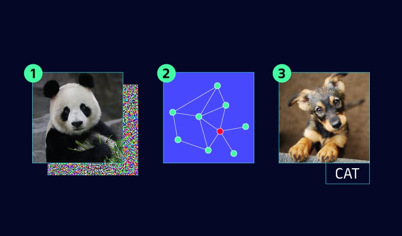
Deep learning is at the center of a new industrial revolution that uses artificial neural networks to create high-performing thinking machines. We are now at the point where machines are becoming better at some tasks than humans, which will revolutionize several major areas of society. This article highlights three hot deep learning areas: adversarial attacks, latent diffusion models, and graph neural networks. Following the excitement of the release of ChatGPT, we want to make sure that you did not overlook some of the other great developments that took place in 2022.
Adversarial models, as their name suggests, take advantage of neural networks. As deep learning models become increasingly relied upon in critical applications such as healthcare, autonomous driving, and cyber security, so does their vulnerability to adversarial attacks.
Latent Diffusion Models are a class of latent variable models that learn the latent structure of a dataset, by modeling the way data points diffuse through the latent space. They can be used to generate images and increase image resolutions.
Graph Neural Networks are a type of artificial neural model that has the potential to revolutionize deep learning. These networks have a flexible structure and can be applied to a broader range of problems that neural networks could not previously solve.
Brace yourself for the future of neural hacking, art, and decision-making!
Adversarial Attacks
Neural networks are now widely accepted as the industry standard for image classification. Currently, neural models are capable of providing near-perfect accuracy in most image classification tasks, including in the ImageNet competition. However, as classification accuracy has increased, so has research into how neural networks function and, more importantly, how they can be broken.
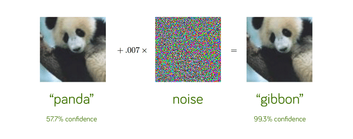
Adversarial attacks involve training a neural network to find and exploit flaws in another neural network. These attacks can prevent a car from detecting stop signs, pedestrians, and even moving. In other cases, they can make people invisible to security cameras.
The most common type of adversarial attack uses gradient-based methods, which exploit backpropagation. Gradient-based attacks take advantage of the backpropagation algorithm by calculating the gradients for a specific input (i.e. image pixels) on a pre-trained network. Using those gradients, a perturbation vector is built, which can be used on input samples to misguide the model.
Some examples of gradient-based methods are as follows:
- Jacobian Saliency Map Attack (JSMA) – uses a greedy algorithm to iteratively change each pixel in an image, as to increase the targeted misclassification (more in this paper)
- Fast Sign Gradient Method (FGSM) – generates an adversarial image by introducing a pixel-wide magnitude perturbation in the approximate gradient direction in a single iteration (more in this paper);
- Carlini-Wagner Attack – Claimed to be stronger than FGSM and JSMA, uses a loss function to measure how well an adversarial sample will be misclassified to an incorrect target label. It does this by finding the minimum difference to create adversarial samples using binary search (more in this paper).
In simple terms, adversarial attacks are optimization techniques, used to mislead a neural network. Here are a few papers that use other techniques to fool neural networks:
- Spoofing road signs: Deep learning models can be easily duped by stickers placed on road signs that can potentially alter the speed limit or cause an autonomous vehicle to run off the road or have other potentially dangerous consequences.
- Spoofing road markings: A joke played on a self-driving car rendered it unable to move. All the attack required was an outer circle of a broken line followed by an inner circle of a continuous line and the vehicle was “trapped” like a bird. As a result, the car “thought” it was allowed to pass through to the inner circle (due to the broken line), but it was unable to exit since it now saw the continuous line.
- Exploiting a face identification algorithm: In this case, researchers created a pair of glasses that led the model to believe that anyone wearing them was Jenifer Lopez. Imagine becoming a superstar using just one pair of glasses.
Although perhaps amusing, these examples show the need to build robust algorithms that can withstand these types of attacks. Fortunately, there are ways in which you can improve the model’s resilience against these attacks by adding adversarial samples to your dataset and retraining it.
Latent Diffusion Models
Some people in the arts community are adamant that artificial intelligence will never replace human-made art because it lacks emotion and other forms of divine inspiration. In reality, neural networks are actually capable of learning how to be artists. This was proven by an AI winning an art competition.
This type of neural model learned to generate art and images based on text input. Simply “say the word,” and this network will paint you a picture in the style of Picasso, Michelangelo, or other world-renowned painters. If you can describe it in words, it can generate it. This technique is known as Diffusers or Latent Diffusion Models, and it will undoubtedly revolutionize the creation of visual content around the world.
StabilityAI developed a model called Stable Diffusion and made it freely available to the public on August 22nd, 2022 – and you can also test it. When it comes to generating high-quality images that are also much more realistic, this new model outperforms Generative Adversarial Networks and auto-regressive techniques like DALL-E.
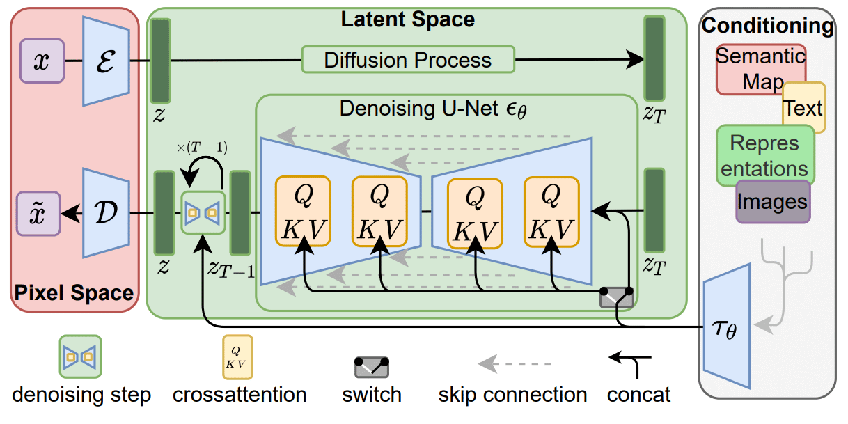
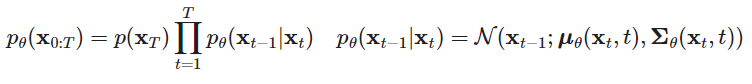
Stable Diffusion is based on an image generation technique known as the latent diffusion model (LDM), which works by iteratively denoising the latent representation space of an image and then decoding that representation to generate a new image. Latent Diffusion Models are probabilistic models designed to learn a data distribution p(x) by gradually denoising a normally distributed variable, which corresponds to learning the reverse process of a fixed Markov Chain of length “T”.
The first step is the forward diffusion, where a small amount of Gaussian noise is iteratively added to the image. When this step is done, you can then apply the reverse diffusion process, which iteratively denoises that input image, creating a new image.
The forward diffusion process adds a small amount of Gaussian noise to a given input sample in T steps, given a data point sampled from a real data distribution x0~q(x). This results in a sequence of noisy samples x1,x2, … , xT, in which the step sizes are controlled by a variance schedule defined by {t(0,1)}t=1T. The full formula for this step can be seen below.

Due to the added noise, the initial sample “ x0” is gradually losing any distinguishing feature it may have, as the step parameter “t” gets larger. When T it means that xT is equivalent to an isotropic Gaussian distribution since its covariance matrix is equal to the identity matrix.
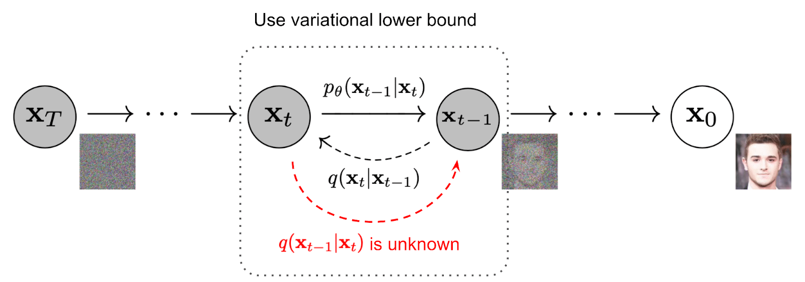
For the reverse diffusion process, we need to reverse the forward diffusion process. We do this by sampling from q(xt-1|xt) so that we recreate the true sample from a Gaussian noise input, xT~Ɲ(0,I).
If t is small enough in this case, the q(xt-1|xt) will also be Gaussian. We now need to learn the model parameters p to run the reverse diffusion model, by approximating conditional probabilities.
The image can now be reconstructed, from the Gaussian noise generated in forward diffusion, to a new sample representing the generated image. Both the forward diffusion and the reverse diffusion are visually represented below.
Now that you know how it works, you can test out the Stable Diffusion algorithm of StabilityAI, by following this link. You can also test StabilityAI’s commercially available version called Dream Studio, which is much better. Finally, here is a nice music video you can watch, where each verse is a computer-generated image.
Graph Neural Networks
Graphs are used all around us. If you ever used Waze or Google Maps to navigate, the shortest route is calculated using a graph. If you use social media like Facebook, the social connections there are also represented as graphs. And, guess what – the Internet is also a huge graph.
The downside of graphs is that they cannot be used well with machine learning, as most algorithms expect a fixed number of inputs and have a fixed structure. Graphs come in different structures and sizes and cannot conform to the fixed structure that classic neural networks expect.
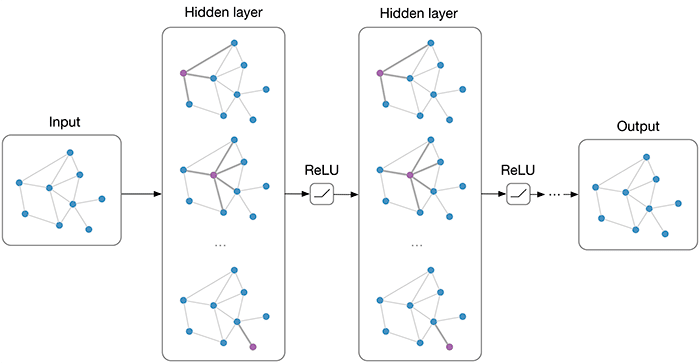
Graph neural networks are the solution, as they are flexible when it comes to both input data and their structure. You can design a neural network just the way you need it, to solve any problem that can be described as a graph.
There are multiple types of graph neural networks out there, but the most important ones are Graph Convolutional Neural Networks (GCNN) and Graph Recurrent Neural Networks (GRNN).
GCNN is a type of graph neural network that uses mechanisms of convolutional neural networks. There are two types of GCNN: spectral and spatial. Spectral networks define graph convolutions by introducing filters from the perspective of graph signal processing which is based on graph spectral theory. Spatial networks formulate graph convolutions as aggregating feature information from neighbors.
The second important type, GRNN, combines the recurrent hidden state that is found in recurrent networks together with Graph Signal Processing. These networks are used when the data can’t be processed by classic RNN due to its structure, the formulation of the problem, or when the data exhibits a time dependency.
The flexibility provided by graph neural networks is both an advantage and a disadvantage. More flexibility makes the time and space complexity of the neural network much higher. This means that training uses up more resources and takes longer. Despite this fact, GNN can solve some problems that other neural networks find impossible to solve.
The Transformer architecture can be seen as a special case of Graph Neural Networks with multi-head attention, treating the sentence as a fully connected graph. Transformers are currently the best-performing technique in Natural Language Processing (NLP) and shook the world with the latest release of ChatGPT.
Graph neural networks have other interesting applications in natural language processing (NLP), where they can be applied to perform text classification for example. A GCNN can be used to convert text into a graph of words, which can then be used to perform reasoning. This type of network has the advantage of capturing semantics and connections between sentences that are very far apart.
In December 2022, at CASP15, the most successful participants leveraged AlphaFold, a game-changing graph neural network that was able to provide structure predictions for nearly all of the proteins known to science. This solved a 50-year-old problem in biology.
Of course, there are various other applications where graph neural networks have the potential to perform well. Some of those are combinatorial optimization, object detection, image classifications, machine translation, and social media recommendation systems.
Graph neural networks have seen increased research in recent years. There is a good chance that we will see more graph neural networks in the future, as they are flexible and can be adapted to tasks that other neural networks cannot solve.
Conclusion
There has been a surge of investment in Deep Learning research and commercialization, due to its potential to solve complex problems across a wide spectrum of industries. However, a major challenge in Deep Learning is the lack of understanding of how neural networks function internally and the lack of testing and analysis in the development process, which can lead to model failures once deployed and a lack of trust.
Tensorleap enables data scientists to improve their models and mitigate the risk of failures with a variety of explainability and debugging tools for Deep Learning models. By incorporating Tensorleap into the development process and increasing explainability in neural networks, we will help drive more innovations in 2023 and beyond.