Question & Answering Problem with the Albert Model
Introduction
This blog will illustrate different explainability methods, focusing on natural language processing (NLP). You will learn how Applied Explainability techniques increase NLP models’ transparency, making them more credible and faster to develop.
Task Overview
Model
I use the ALBERT, introduced in ALBERT: A Lite BERT for Self-supervised Learning of Language Representations by Zhenzhong Lan et al. The model was trained on the Stanford Question Answering Dataset (SQuAD) 1.1, a collection of questions and answers from Wikipedia articles. (base, E=128: F1=89.3, EM=82.3)
Input
In the Question Answering (QA) task, the model’s input consists of the question and a section (a.k.a. The context) from which the model will detect the answer. See the example below:
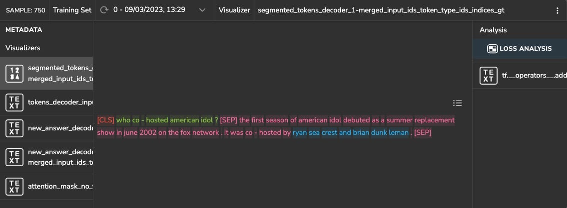
In this example, you can see that the question is separated by the “[SEP]” token, followed by the context, and that the model correctly predicted the answer to the question “Who co-hosted American Idol?” (highlighted in green), as “Ryan Seacrest and Brian Dunkleman.”
Output
The model’s output is a multi-prediction composed of two predictions: the start and end indexes of the answer within the text (context). The projections are a classification of a fixed sequence length of the index. Accordingly, the ground truth consists of two one-hot encoded vectors with a fixed sequence length K, denoted by: [0,1]k
Interpreting the Model with Applied Explainability
Latent Space Exploration
To better understand the model and see where the model may be failing, I construct a latent space from the model’s most informative features. Rather than do it manually, which could be pretty time-consuming, I use Tensorleap to automatically create the latent space—which involves projecting the most informative features of the model into a two-dimensional space.
This latent space captures meaningful and semantic information interpreted by the model. The sample topology projected on that latent space can help us gain insights into the model’s outputs and identify hidden patterns. By visualizing external variables along with the visualization of the latent space, we can identify possible correlations between our model’s interpretations and the variables. Moreover, identifying such correlations that may impact the model’s performance enables us to address them accordingly.
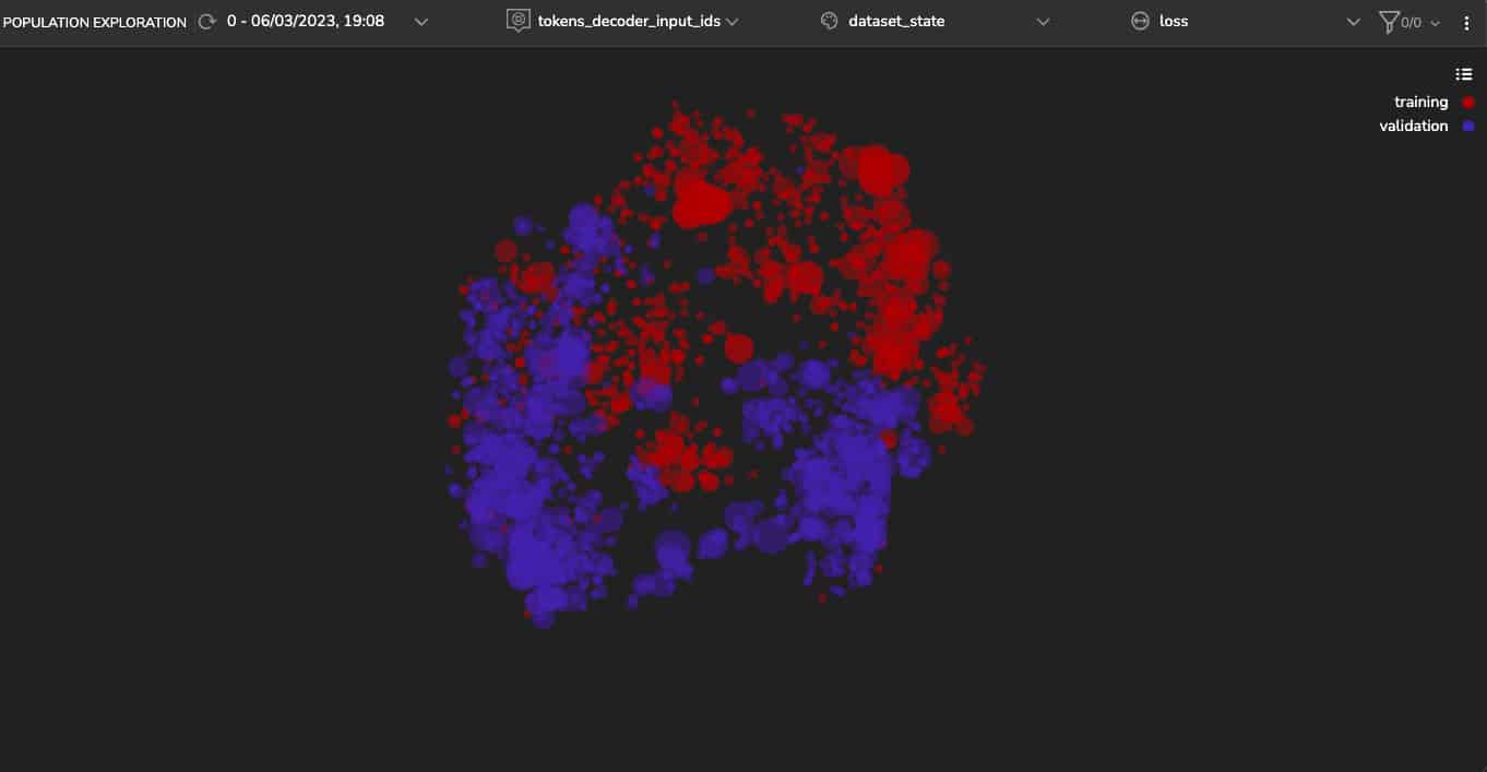
For example, Figure 2 shows a visualization of the training and validation sets in a shared latent space where we can see two distinct clusters. This means there is a difference in their representation—either the model does not perform well and overfits, or there’s a significant difference in the data. We know that the model’s generalization capability isn’t an issue, so we will investigate other factors that may have contributed to this behavior.
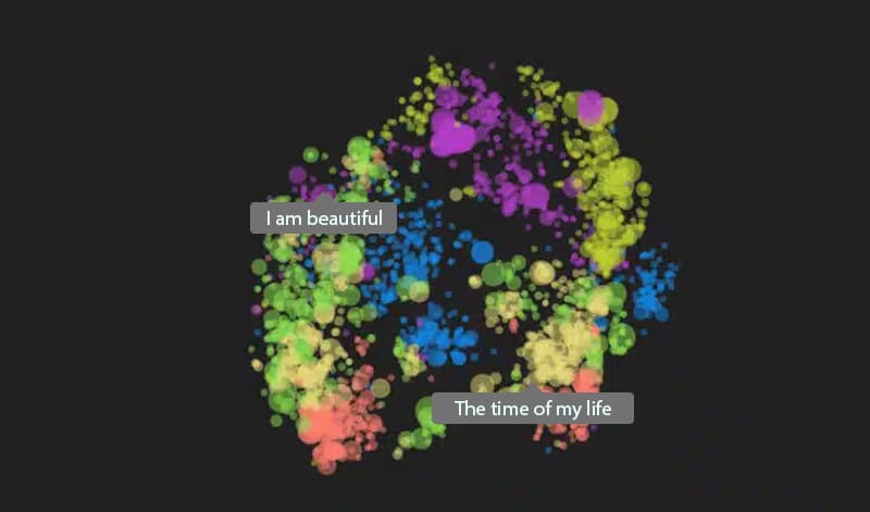
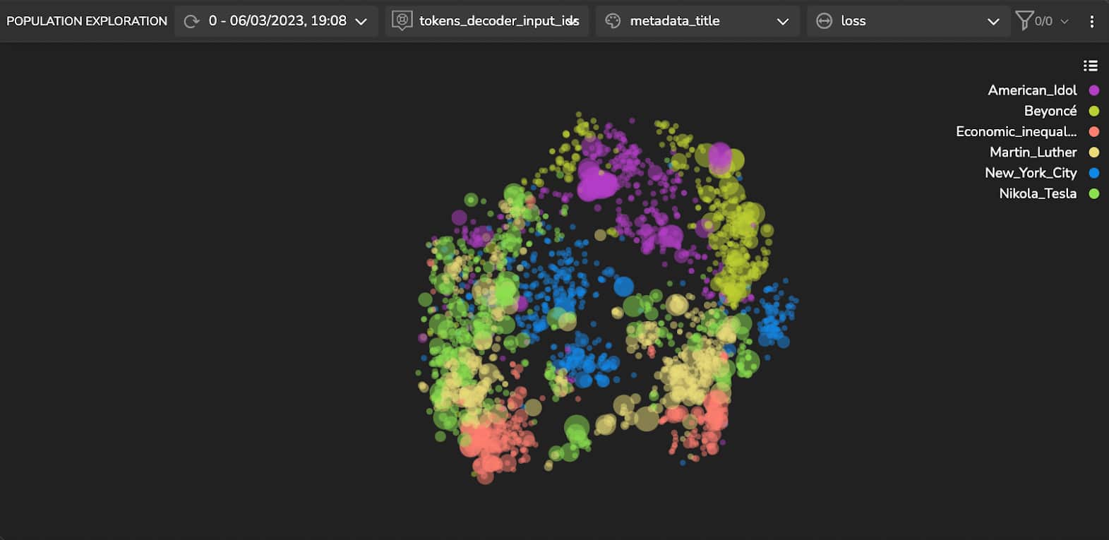
In SQuAD, the samples in the training and validation sets relate to different topics. Therefore, it is reasonable to presume that the other sets have distinct features and characteristics. We hypothesize that this is the reason that the model represents them as distinct clusters. To quickly try this hypothesis, we color the samples’ according to their topic (Figure 3). We can see that the latent space’s spread is indeed correlated to the topic of the samples.
Detecting & Handling High Loss Clusters
Further analysis of Figure 3 reveals that a cluster in the ‘American Idol’ samples has a higher loss (larger dot sizes). At a glance, we can see that this cluster contains questions that relate to the names of songs (Figures 4a and 4b), such as “what was [singer’s name] first single?” or “what is the name of the song…?”.
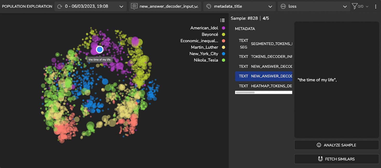
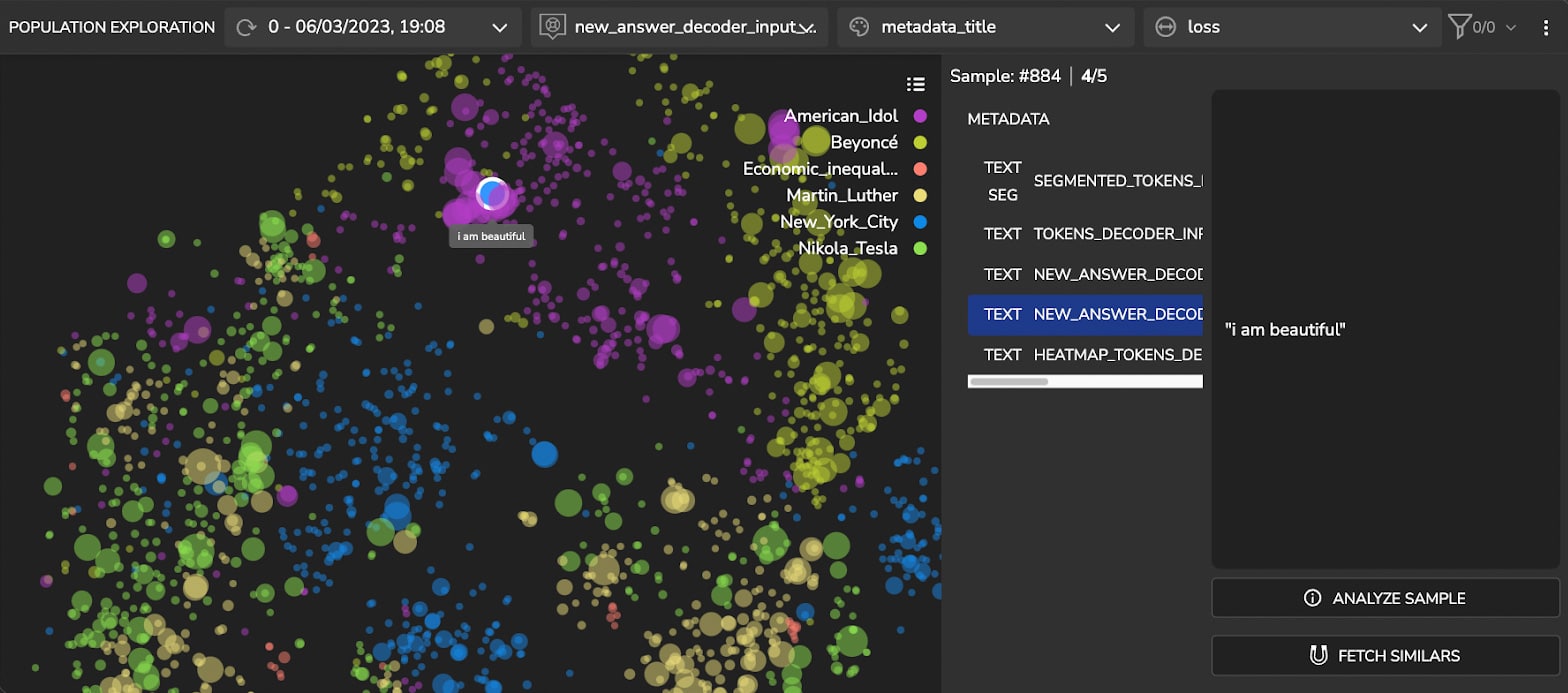
It appears that the model did detect the correct answers. However, the prediction contains quotation marks while the ground truth doesn’t. See Figure 5 below. To address this discrepancy, we tweak our decoding function.
Detecting Unlabeled Clusters in the Latent Space
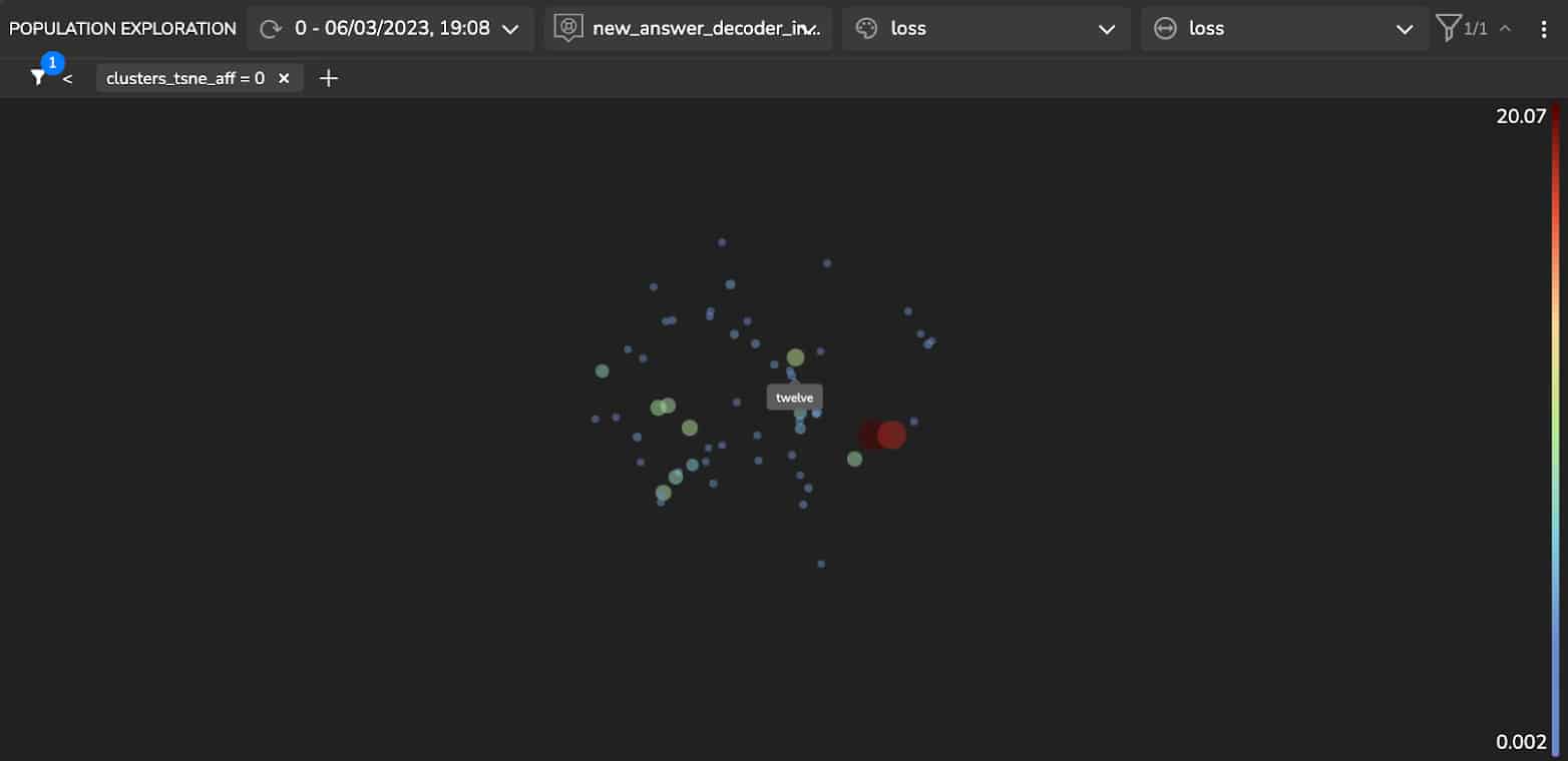
Now, let’s look for additional clusters in our data using an unsupervised clustering algorithm on the model’s latent space. Here we show clusters detected using the Affinity Propagation (AP) algorithm (see Figure 5).
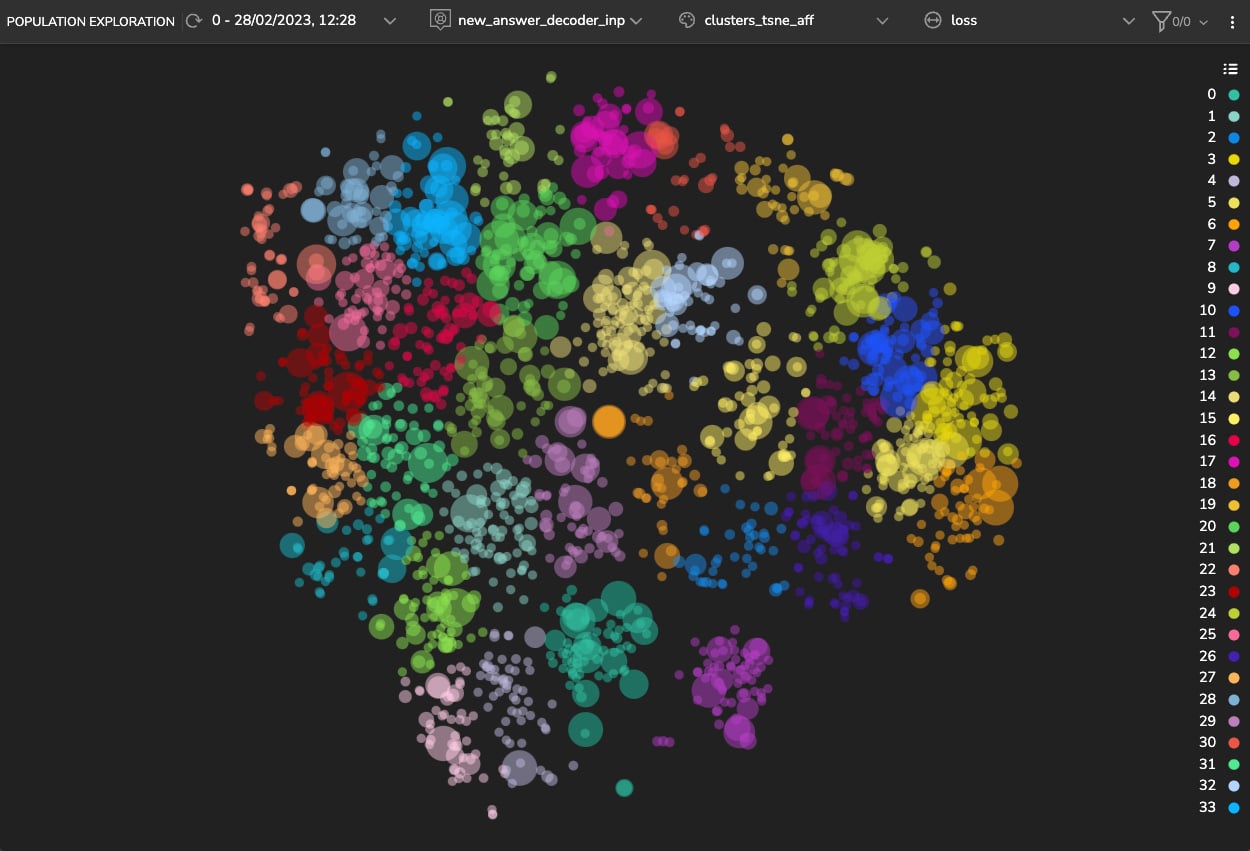
Upon examination of these clusters, we can see the following:
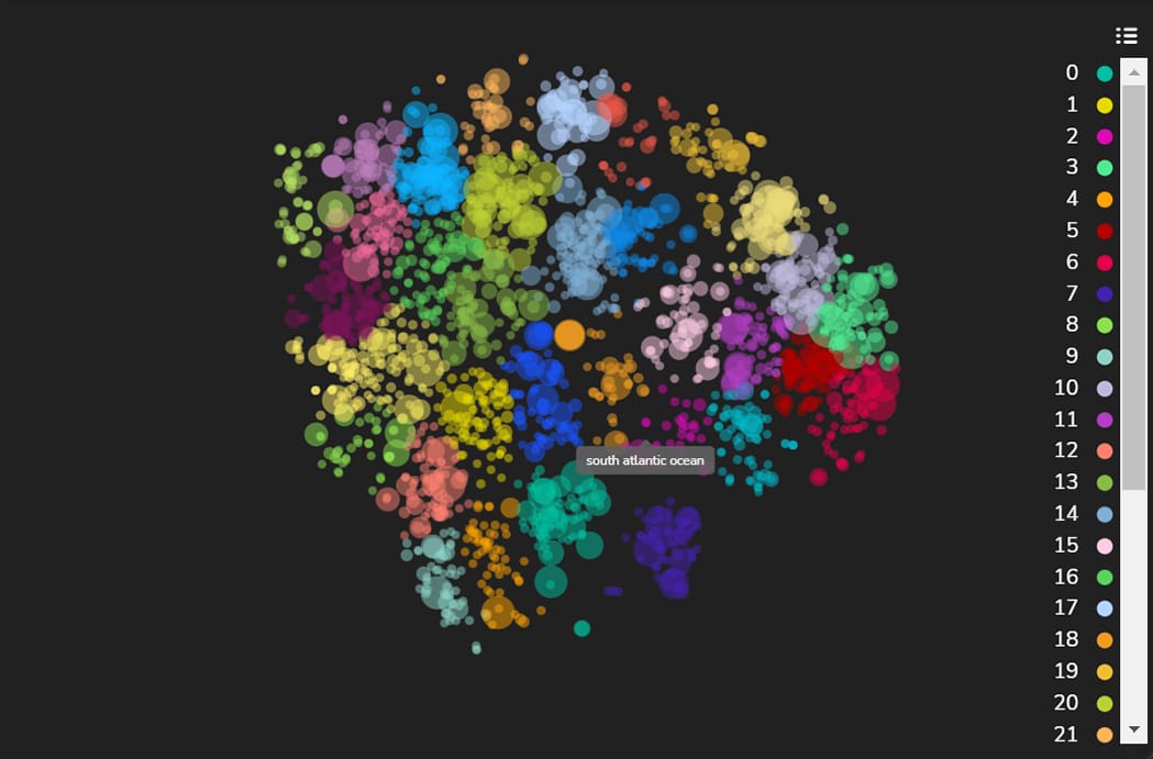
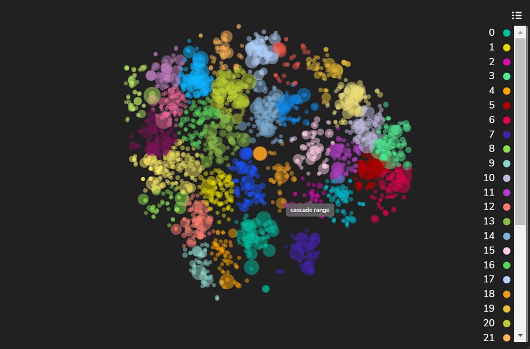
- Cluster 2 includes answers that relate to geographic locations such as “Gulf of Mexico”, “Texas”, “Hawaii” etc.

Figure 6a: A cluster of answers that relate to locations—Hawaii
Figure 6b: A cluster of answers that relate to locations—South Atlantic Ocean
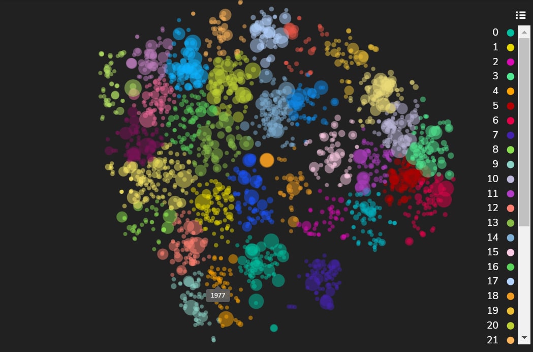
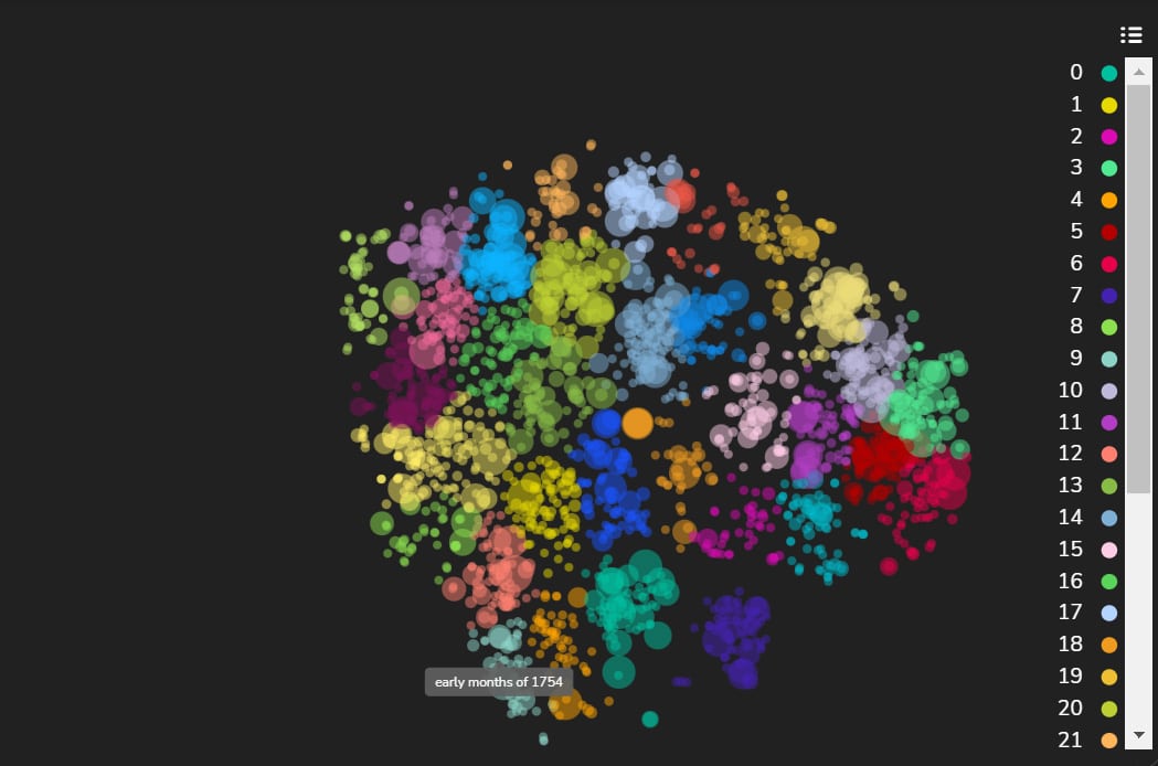
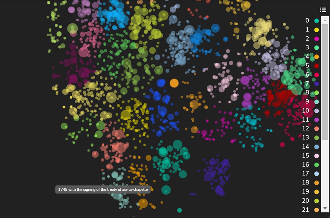
Figure 6c: A cluster of answers that relate to locations—Cascade Range - Clusters 4 and 9, located close to each other, contain answers relating to years and dates of events. Cluster 4 includes primarily questions that require answers related to years, such as “What year…?” where the answers are years represented in digits: “1989”, “1659” etc. Cluster 9, shown in Figure 8, includes questions that require answers related to dates and times, such as “When.. ?” and answers of the dates and times represented in text and digits: “early months of 1754”, “1 January 1926”, “end of October 2006”, “1990s” etc.

Figure 7a: Answers to Questions that Require the Year of the Event—1977
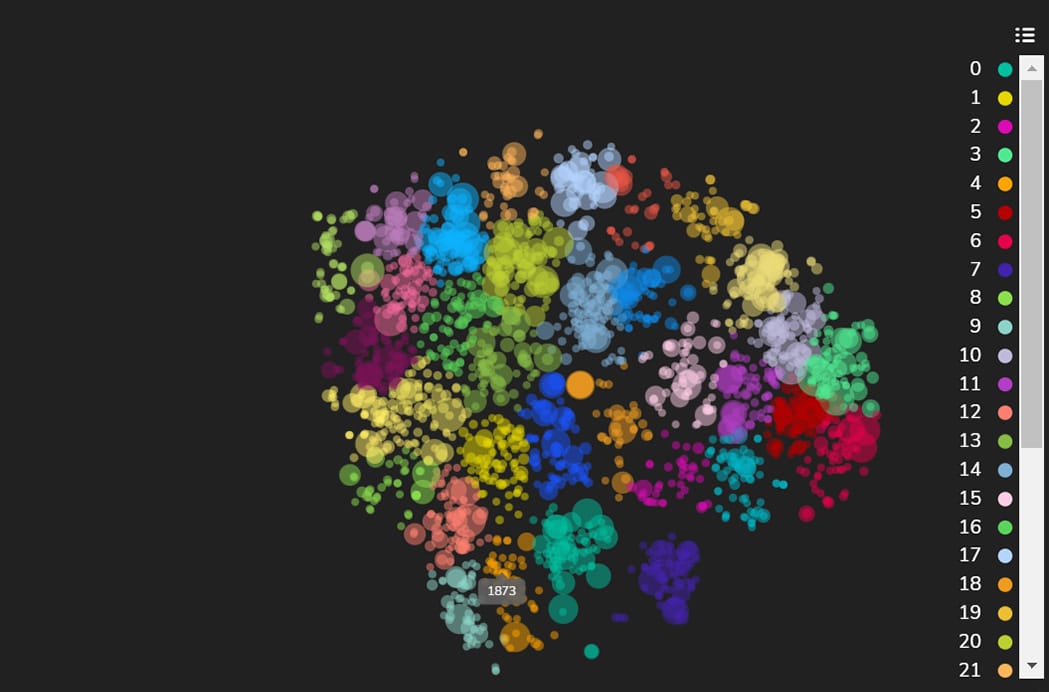
Figure 7b: Answers to Questions that Require the Year of the Event—1873
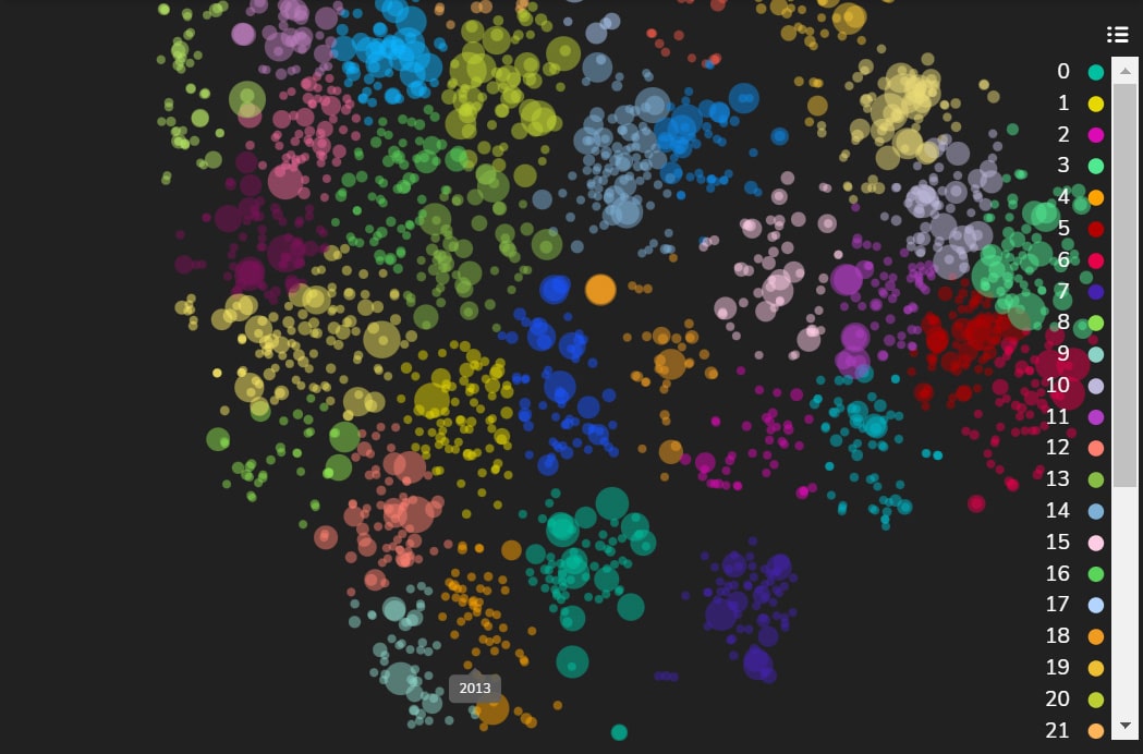
Figure 7c: Answers to Questions that Require the Year of the Event—2013 
Figure 8a: Answers that Require the Date of the Event—Early Months of 1754
Figure 8b: Answers that Require the Date of the Event—Signing of the Treaty of Aix-La Chapelle
Figure 8c: Answers that Require the Date of the Event—Early 2018


Another approach to finding clusters using the model’s latent space is fetching similar samples to a selected sample. It enables you to identify a cluster with an intrinsic property you want to investigate. The similarity is based on its feature representations in that model’s latent space. By detecting this cluster, you can gain insights into how the model interprets this sample and, in general, retrieve clusters with more abstract patterns.
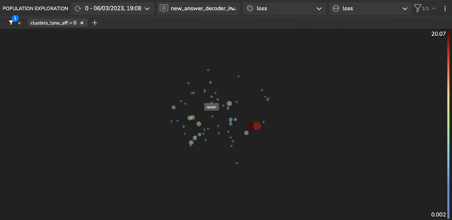
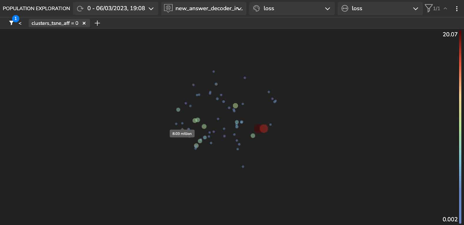
Figure 9 shows a Quantitative Questions and Answers cluster. We can see that the cluster which includes quantitative questions and answers contains questions such as “How many …?”, “How often…?”, “How much …?” and answers represented in digits and in words: “three”, “two”, “4%”, “50 million”, “many thousands”.
Sample Loss Analysis
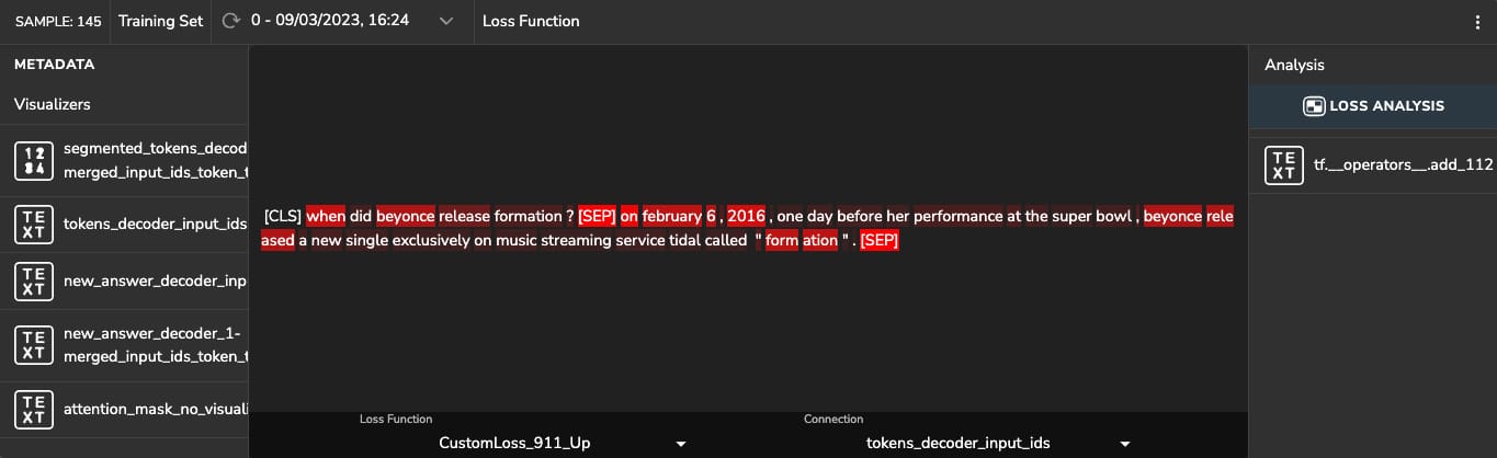
In this section, we can see the results of a gradient-based explanatory algorithm to interpret what drives the model to make specific predictions. Extracting the model’s most important features and calculating derivatives of the loss function with respect to the activation maps enables us to analyze which of the informative features contributes most to the loss function. We then generate a heatmap with these features that shows the relevant information.
Let’s analyze the following sample containing the question: “when did Beyonce release ‘formation’?”. The correct predicted answer is: “February 6, 2016”. We see that the tokens that had the most impact on the model’s prediction are: ‘when’, ‘beyonce’, ‘release’, ‘released’, ‘formation’. Also the answer tokens:’ february’, ‘6’,’ 2016′, and the ‘[SEP]’ token.
False / Ambiguous Labeling
This section illustrates inaccurate and mislabeled samples.
Figure 11 shows a sample with the question, “The first successful water landing in the Indian Ocean by the Soviets was when?” (shown in green). The correct answer to this question is 1968. Although the ground truth indexes refer to the correct token values, they were labeled in an incorrect and unrelated location: “..during the summer of 1968, the Apollo program hit another snag: the first pilot…” (in yellow). The model correctly predicted the answer’s indexes, which are located in the right context sentence: “In September 1968, zond5 made a circumlunar flight… accomplishing the first successful water landing of the Soviet space program… “(in purple).
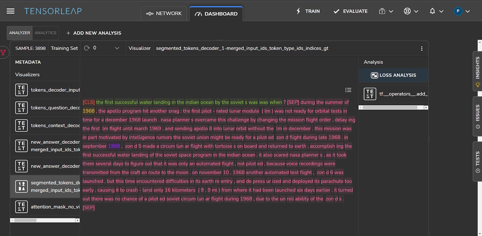
Figure 12 shows a sample with the question (shown in green): “Did Tesla graduate from the university?” The answer from the context is: “he never graduated from the university” (shown in purple). This was detected correctly by the model. However, the ground truth’s indexes refer to “no” (shown in yellow) in the sentence: “no Sundays or holidays…”. As in the above example, the indexes are incorrect and in an unrelated location to the question.
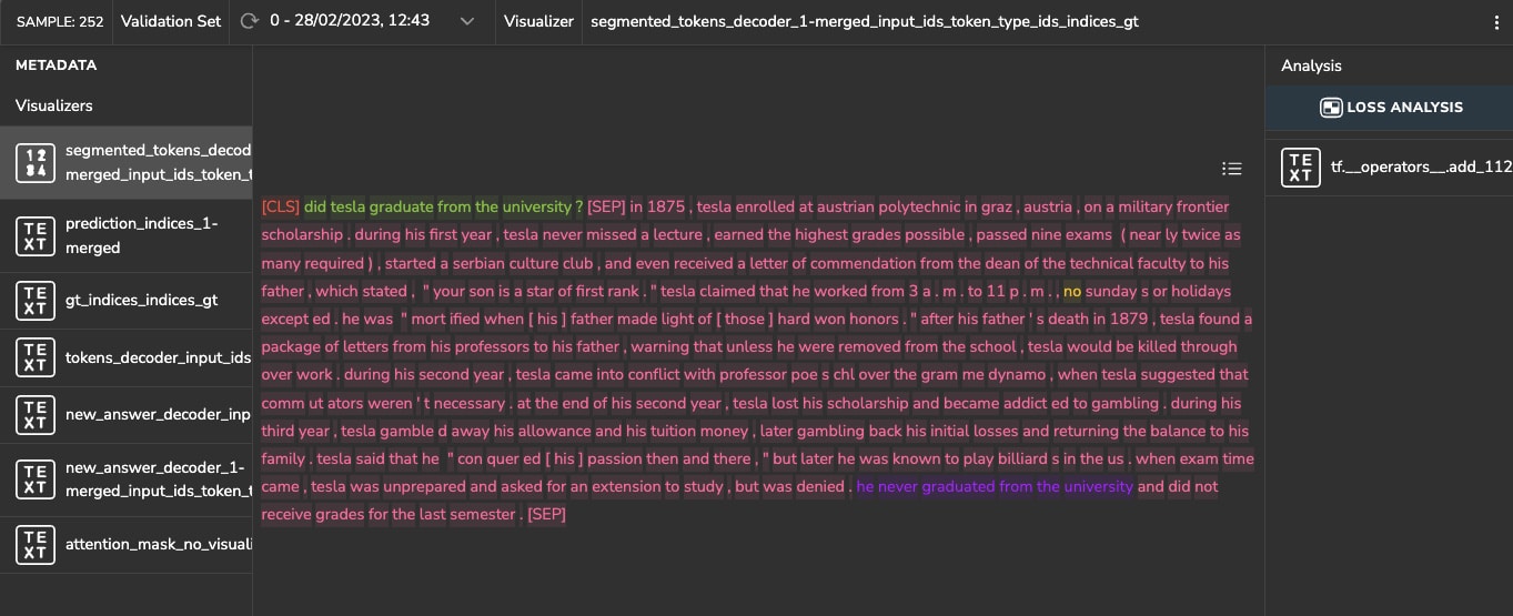
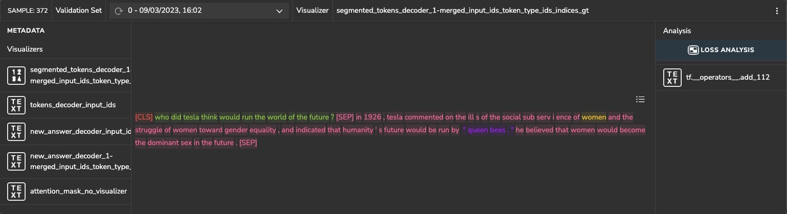
Figure 13 shows a sample with the question: “Who did Tesla think would run the world of the future?” (shown in green). Again, the ground-truth indexes are located in unrelated and inaccurate locations: “… on the ills of the social subservience of women“, while the model prediction refers to the correct context location: “… humanity’s future would be run by ‘queen bees'”.
Such cases distort the model’s performance and negatively affect its fitting when penalizing the model on these samples. We can solve these issues by changing the ground truth or by removing such samples.
Conclusion
I leveraged an informative latent space in this article to qualitatively evaluate and obtain insights on a language model. I showcased Applied Explainability techniques on the Question Answering (QA) task utilizing the SQuAD dataset and the Albert transformer-based model.
By exploring such a latent space, you could see how we can easily detect unlabeled clusters and handle those with high loss. I demonstrated different clustering approaches and Applied Explainability techniques. At the sample level, I showed an example of loss analysis and how it might help us to understand the model’s predictions. In addition, I found some labeling-related issues in our data.
Without the automatic generation of the informative latent space and additional Tensorleap analytic tools, drawing the conclusions discussed in this article would have demanded a great deal of time-consuming manual work.